Note
Download this Jupyter notebook and all
data
(unzip next to the ipynb file!).
You will need a Gurobi license to run this notebook, please follow the
license instructions.
Investing with Transaction Costs
The standard mean-variance (Markowitz) portfolio selection model determines an optimal investment portfolio that balances risk and expected return. In this notebook, we maximize the portfolio’s expected return while constraining the admissible variance (risk) to a given maximum level. Please refer to the annotated list of references for more background information on portfolio optimization.
To this basic model, we add transaction costs and fees. These have two components:
Fixed transaction costs, which are independent of the amount invested in each separate asset.
Variable transaction fees, which are proportional to the amount invested in each asset.
This notebook focuses on constructing a new portfolio and assumes that the investor has no initial positions.
[2]:
import gurobipy as gp
import pandas as pd
import numpy as np
import matplotlib.pyplot as plt
Input Data
The following input data is used within the model:
\(S\): set of stocks
\(\mu\): vector of expected returns
\(\Sigma\): PSD variance-covariance matrix
\(\sigma_{ij}\) covariance between returns of assets \(i\) and \(j\)
\(\sigma_{ii}\) variance of return of asset \(i\)
[4]:
# Import some example data set
Sigma = pd.read_pickle("sigma.pkl")
mu = pd.read_pickle("mu.pkl")
Formulation
The model creates a new portfolio (no initial positions held by the investor) by maximizing the expected net return while ensuring that the variance of the portfolio return does not exceed a specified level. It also accounts for the impact of transaction costs on the available investment budget.
The transaction costs are twofold:
The fixed transaction costs for buying each asset, which do not depend on the amount invested.
The variable transaction fees, which are proportional (also called linear) to the amount invested into each asset.
Mathematically, this results in a convex quadratically constrained mixed-integer optimization problem.
Model Parameters
We use the following parameters:
\(\bar\sigma^2\): maximal admissible variance for the portfolio return
\(\ell>0\): lower bound on position size
\(c\): fixed transaction costs for any asset, relative to total investment value
\(f_i\): variable transaction fee for asset \(i\), relative to total investment value
In this notebook, we assume that the fixed costs are the same for each asset, while the variable fees may differ for different assets. Both costs and fees are given relative to the total capital.
[5]:
# Values for the model parameters:
V = 4.0  # Maximal admissible variance (sigma^2)
l = 0.001  # Minimal position size
c = 0.0001  # Fixed transaction costs
f = 0.001 * np.ones(mu.shape)  # Variable transaction fees
Decision Variables
We need two sets of decision variables:
The proportions of capital invested among the considered stocks. The corresponding vector of positions is denoted by \(x\) with its component \(x_i\) denoting the proportion of capital invested in stock \(i\).
Binary variables \(b_i\) indicating whether or not asset \(i\) is held. If \(b_i\) is 0, the holding \(x_i\) is also 0; otherwise if \(b_i\) is 1, the investor holds asset \(i\) (that is, \(x_i \geq \ell\)).
Variable Bounds
Each position must be between 0 and 1; this prevents leverage and short-selling:
The \(b_i\) must be binary:
[6]:
%%capture
# Create an empty optimization model
m = gp.Model()

# Add variables: x[i] denotes the proportion invested in stock i
x = m.addMVar(len(mu), lb=0, ub=1, name="x")

# Add variables: b[i]=1 if stock i is held, and b[i]=0 otherwise
b = m.addMVar(len(mu), vtype=gp.GRB.BINARY, name="b")
Constraints
The estimated risk must not exceed a prespecified maximal admissible level of variance \(\bar\sigma^2\):
[7]:
%%capture
# Upper bound on variance
m.addConstr(x @ Sigma.to_numpy() @ x <= V, name="Variance")
From the bounds we set earlier, \(x\) can take any value between \(0\) and \(1\). To enforce the desired relationship between \(x\) and the binary variables \(b\), we use the following sets of discrete constraints:
Ensure that \(x_i = 0\) if \(b_i = 0\): \begin{equation*} x_i \leq b_i \; , \; i \in S\tag{1} \end{equation*}
Note that since \(x_i\) has an upper bound of 1, the above constraint is non-restrictive when \(b_i = 1\).
Ensure a minimal position size of \(\ell\) if asset \(i\) is traded: \begin{equation*} x_i \geq \ell b_i \; , \; i \in S\tag{2} \end{equation*}
Hence \(b_i = 1\) implies \(x_i \geq \ell\). Additionally, if \(b_i = 0\), the above constraint is non-restrictive since \(x_i\) has a lower bound of 0.
[8]:
%%capture
# Force x to 0 if not traded; see formula (1) above
m.addConstr(x <= b, name="Indicator")
# Minimal position; see formula (2) above
m.addConstr(x >= l * b, name="Minimal_Position")
Without any costs or fees, we would have the budget constraint \(\sum_{i} x_i = 1\) to ensure that all investments sum up to one. However, we must also deduct the resulting fixed transaction costs and variable transaction fees from the capital.
The fixed costs are incurred whenever an asset is held and do not depend on the position size; hence, the fixed cost for each asset \(i\) is \(cb_i\). The variable fees are proportional to the position size; hence, the fee for each asset \(i\) is \(f_ix_i\).
We include these in the left-hand side of the equation:
\begin{equation*} \underbrace{\sum_{i \in S} x_i}_\text{investments} + \underbrace{c \sum_{i \in S} b_i}_\text{fixed costs} + \underbrace{\sum_{i \in S}f_i x_i}_\text{variable fees} = 1 \tag{3} \end{equation*}
[9]:
# Budget constraint: all investments, costs, and fees sum up to 1; see formula (3) above
budget_constr = m.addConstr(
    x.sum() + b.sum() * c + f @ x == 1, name="Budget_Constraint"
)
Objective Function
The objective is to maximize the expected return of the portfolio:
[10]:
# Define objective: Maximize expected return
m.setObjective(mu.to_numpy() @ x, gp.GRB.MAXIMIZE)
We now solve the optimization problem:
[11]:
m.params.mipgap = 0.01
m.optimize()
Set parameter MIPGap to value 0.01
Gurobi Optimizer version 13.0.2 build v13.0.2rc1 (linux64 - "Ubuntu 24.04.4 LTS")

CPU model: AMD EPYC 7763 64-Core Processor, instruction set [SSE2|AVX|AVX2]
Thread count: 1 physical cores, 2 logical processors, using up to 2 threads

Non-default parameters:
MIPGap  0.01

WLS license 2443533 - registered to Gurobi GmbH
Optimize a model with 925 rows, 924 columns and 2772 nonzeros (Max)
Model fingerprint: 0xa1c281a1
Model has 462 linear objective coefficients
Model has 1 quadratic constraint
Variable types: 462 continuous, 462 integer (462 binary)
Coefficient statistics:
  Matrix range     [1e-04, 1e+00]
  QMatrix range    [3e-03, 1e+02]
  Objective range  [7e-02, 6e-01]
  Bounds range     [1e+00, 1e+00]
  RHS range        [1e+00, 1e+00]
  QRHS range       [4e+00, 4e+00]

Presolve time: 0.10s
Presolved: 925 rows, 924 columns, 2772 nonzeros
Presolved model has 1 quadratic constraint(s)
Variable types: 462 continuous, 462 integer (462 binary)

Root relaxation: objective 5.914499e-01, 3 iterations, 0.00 seconds (0.00 work units)

    Nodes    |    Current Node    |     Objective Bounds      |     Work
 Expl Unexpl |  Obj  Depth IntInf | Incumbent    BestBd   Gap | It/Node Time

     0     0    0.59145    0    2          -    0.59145      -     -    0s
     0     0    0.56243    0    2          -    0.56243      -     -    0s
H    0     0                       0.2724533    0.56238   106%     -    0s
H    0     0                       0.3089999    0.56238  82.0%     -    0s
H    0     0                       0.3188252    0.56238  76.4%     -    0s
H    0     0                       0.3197091    0.56238  75.9%     -    1s
H    0     0                       0.3233401    0.56238  73.9%     -    1s
H    0     0                       0.3241527    0.56238  73.5%     -    1s
H    0     0                       0.3241703    0.56238  73.5%     -    1s
H    0     0                       0.3245174    0.56238  73.3%     -    1s
H    0     0                       0.3247104    0.56238  73.2%     -    1s
H    0     0                       0.3248003    0.56238  73.1%     -    1s
H    0     0                       0.3248414    0.56238  73.1%     -    1s
H    0     0                       0.3248423    0.56238  73.1%     -    1s
     0     0    0.43869    0    3    0.32484    0.43869  35.0%     -    1s
     0     0    0.43863    0    4    0.32484    0.43863  35.0%     -    1s
     0     0    0.42948    0    4    0.32484    0.42948  32.2%     -    1s
     0     0    0.42853    0    5    0.32484    0.42853  31.9%     -    1s
     0     0    0.41286    0    5    0.32484    0.41286  27.1%     -    1s
     0     0    0.41284    0    5    0.32484    0.41284  27.1%     -    1s
     0     0    0.40005    0    5    0.32484    0.40005  23.2%     -    1s
     0     0    0.40005    0    5    0.32484    0.40005  23.2%     -    1s
     0     0    0.39464    0    5    0.32484    0.39464  21.5%     -    1s
     0     0    0.39248    0    6    0.32484    0.39248  20.8%     -    1s
     0     0    0.39233    0    7    0.32484    0.39233  20.8%     -    1s
     0     0    0.38946    0    7    0.32484    0.38946  19.9%     -    1s
     0     0    0.38895    0    8    0.32484    0.38895  19.7%     -    1s
     0     0    0.38786    0    9    0.32484    0.38786  19.4%     -    1s
     0     0    0.38602    0    8    0.32484    0.38602  18.8%     -    1s
     0     0    0.38583    0    9    0.32484    0.38583  18.8%     -    1s
     0     0    0.38280    0    9    0.32484    0.38280  17.8%     -    1s
     0     0    0.38153    0    9    0.32484    0.38153  17.5%     -    1s
     0     0    0.38006    0    8    0.32484    0.38006  17.0%     -    1s
     0     0    0.37949    0    8    0.32484    0.37949  16.8%     -    1s
     0     0    0.37893    0    9    0.32484    0.37893  16.7%     -    2s
     0     0    0.37835    0    9    0.32484    0.37835  16.5%     -    2s
     0     0    0.37807    0   10    0.32484    0.37807  16.4%     -    2s
     0     0    0.37757    0    9    0.32484    0.37757  16.2%     -    2s
     0     0    0.37740    0    9    0.32484    0.37740  16.2%     -    2s
     0     0    0.37682    0   10    0.32484    0.37682  16.0%     -    2s
     0     0    0.37682    0   10    0.32484    0.37682  16.0%     -    3s
     0     0    0.37682    0   10    0.32484    0.37682  16.0%     -    3s
H    0     0                       0.3499460    0.37682  7.68%     -    3s
H    0     0                       0.3506240    0.37682  7.47%     -    3s
H    0     0                       0.3506270    0.37682  7.47%     -    3s
H    0     0                       0.3507253    0.37682  7.44%     -    3s
H    0     0                       0.3507323    0.37682  7.44%     -    3s
H    0     0                       0.3507390    0.37682  7.44%     -    3s
H    0     0                       0.3507465    0.37682  7.43%     -    3s
     0     2    0.37681    0   10    0.35075    0.37681  7.43%     -    4s
    11    13    0.37595   11    2    0.35075    0.37669  7.40%   1.9    5s
H   34    34                       0.3508115    0.37668  7.37%   4.0    5s
H   38    38                       0.3522203    0.37668  6.94%   4.0    5s
H   52    52                       0.3522203    0.37656  6.91%   5.1    5s
H   52    52                       0.3526560    0.37656  6.78%   5.1    5s
H   53    53                       0.3530810    0.37656  6.65%   5.0    6s
H  175   175                       0.3530810    0.37647  6.62%   7.3    8s
H  175   175                       0.3531287    0.37647  6.61%   7.3    8s
H  175   175                       0.3531294    0.37647  6.61%   7.3    8s
   232   221    0.35522   22    1    0.35313    0.37625  6.55%   7.4   10s

Explored 265 nodes (2243 simplex iterations) in 11.24 seconds (11.64 work units)
Thread count was 2 (of 2 available processors)

Solution count 10: 0.353129 0.353129 0.353081 ... 0.350725

Optimal solution found (tolerance 1.00e-02)
Best objective 3.531294334276e-01, best bound 3.536987553827e-01, gap 0.1612%
Display basic solution data, costs, and fees:
[12]:
print(f"Expected return:  {m.ObjVal:.6f}")
print(f"Solution time:    {m.Runtime:.2f} seconds\n")
print(f"Fixed costs:      {c * sum(b.X):.6f}")
print(f"Variable fees:    {f @ x.X:.6f}")
print(f"Number of trades: {sum(b.X)}\n")

# Print investments (with non-negligible value, i.e. >1e-5)
positions = pd.Series(name="Position", data=x.X, index=mu.index)
print(positions[positions > 1e-5])
Expected return:  0.353129
Solution time:    11.25 seconds

Fixed costs:      0.002000
Variable fees:    0.000997
Number of trades: 20.0

TSLA    0.015687
KR      0.028968
PGR     0.129075
ORLY    0.050234
ODFL    0.030784
KDP     0.063330
META    0.013082
UNH     0.020016
AVGO    0.062520
DXCM    0.018539
NFLX    0.021316
LLY     0.247054
DPZ     0.030767
WST     0.021614
TMUS    0.037723
NOC     0.051112
MOH     0.005462
TTWO    0.032825
ENPH    0.010687
NVDA    0.106207
Name: Position, dtype: float64
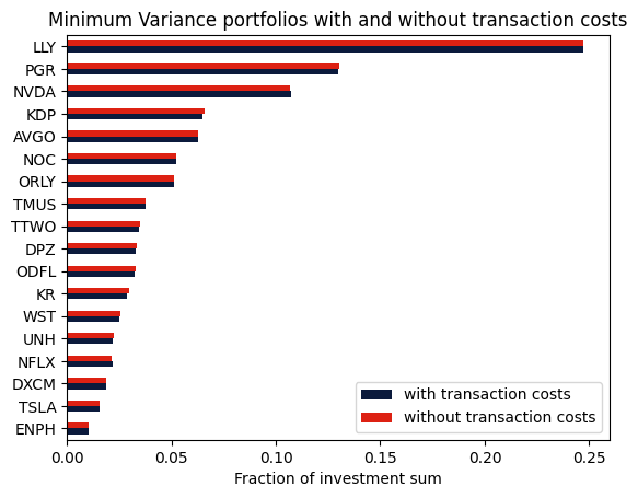
Comparison with the unconstrained portfolio
We can also optimize the portfolio without considering the transaction costs and compare the resulting portfolios.
[13]:
# remove budget constraint
m.remove(budget_constr)
# add new budget constraint without costs
m.addConstr(x.sum() == 1, name="Budget_Constraint")
m.params.OutputFlag = 0
m.optimize()

# retrieve and display solution data
positions_no_costs = pd.Series(name="Position", data=x.X, index=mu.index)
mask = (positions > 1e-5) | (positions_no_costs > 1e-5)
df = pd.DataFrame(
    index=positions[mask].index,
    data={
        "with transaction costs": positions,
        "without transaction costs": positions_no_costs,
    },
).sort_values("with transaction costs", ascending=True)

axs = df.plot.barh(color=["#0b1a3c", "#dd2113"])
axs.set_xlabel("Fraction of investment sum")
plt.title("Minimum Variance portfolios with and without transaction costs")
plt.show()
Takeaways
Transaction costs and fees can be incorporated into the basic budget constraint.
Fixed costs are independent of the traded amount and can be modeled using binary decision variables.
Variable fees are proportional to the traded amount and can be modeled using continuous decision variables.