Note
Download this Jupyter notebook and all
data
(unzip next to the ipynb file!).
You will need a Gurobi license to run this notebook, please follow the
license instructions.
Maximizing Utility
The standard mean-variance (Markowitz) portfolio selection model determines an optimal investment portfolio that balances risk and expected return. In this notebook, we maximize the utility, which is defined as a weighted linear function of return and risk that can be adjusted by varying the risk-aversion coefficient \(\gamma\). Please refer to the annotated list of references for more background information on portfolio optimization.
[2]:
import gurobipy as gp
import pandas as pd
import numpy as np
import matplotlib.pyplot as plt
Input Data
The following input data is used within the model:
\(S\): set of stocks
\(\mu\): vector of expected returns
\(\Sigma\): PSD variance-covariance matrix
\(\sigma_{ij}\) covariance between returns of assets \(i\) and \(j\)
\(\sigma_{ii}\) variance of return of asset \(i\)
[4]:
# Import example data
Sigma = pd.read_pickle("sigma.pkl")
mu = pd.read_pickle("mu.pkl")
Formulation
The model maximizes the investor’s expected utility, which is defined as a linear combination of the expected return and risk, accounting for the investor’s level of risk aversion via the risk-aversion coefficient \(\gamma\). Mathematically, this results in a convex quadratic optimization problem.
Decision Variables and Variable Bounds
The decision variables in the model are the proportions of capital invested among the considered stocks. The corresponding vector of positions is denoted by \(x\) with its component \(x_i\) denoting the proportion of capital invested in stock \(i\).
Each position must be between 0 and 1; this prevents leverage and short-selling:
Constraints
The budget constraint ensures that all capital is invested:
Objective Function
The objective is to maximize expected utility:
Using gurobipy, this can be expressed as follows:
[5]:
%%capture
gamma = 0.2  # risk-aversion coefficient

# Create an empty optimization model
m = gp.Model()

# Add variables: x[i] denotes the proportion invested in stock i
# 0 <= x[i] <= 1
x = m.addMVar(len(mu), lb=0, ub=1, name="x")

# Budget constraint: all investments sum up to 1
m.addConstr(x.sum() == 1, name="Budget_Constraint")

# Define objective function: Maximize expected utility
m.setObjective(
    mu.to_numpy() @ x - gamma / 2 * (x @ Sigma.to_numpy() @ x), gp.GRB.MAXIMIZE
)
We now solve the optimization problem:
[6]:
m.optimize()
Gurobi Optimizer version 13.0.2 build v13.0.2rc1 (linux64 - "Ubuntu 24.04.4 LTS")

CPU model: AMD EPYC 7763 64-Core Processor, instruction set [SSE2|AVX|AVX2]
Thread count: 1 physical cores, 2 logical processors, using up to 2 threads

WLS license 2443533 - registered to Gurobi GmbH
Optimize a model with 1 rows, 462 columns and 462 nonzeros (Max)
Model fingerprint: 0xee0d2d3c
Model has 462 linear objective coefficients
Model has 106953 quadratic objective terms
Coefficient statistics:
  Matrix range     [1e+00, 1e+00]
  Objective range  [7e-02, 6e-01]
  QObjective range [6e-04, 2e+01]
  Bounds range     [1e+00, 1e+00]
  RHS range        [1e+00, 1e+00]

Presolve time: 0.02s
Presolved: 1 rows, 462 columns, 462 nonzeros
Presolved model has 106953 quadratic objective terms
Ordering time: 0.01s

Barrier statistics:
 Free vars  : 461
 AA' NZ     : 1.065e+05
 Factor NZ  : 1.070e+05 (roughly 1 MB of memory)
 Factor Ops : 3.298e+07 (less than 1 second per iteration)
 Threads    : 1

                  Objective                Residual
Iter       Primal          Dual         Primal    Dual     Compl     Time
   0  -2.00616666e+05  3.17727204e+05  2.51e+05 6.60e-01  2.50e+05     0s
   1  -5.25149343e+04  5.58459714e+04  6.22e+03 8.36e-06  6.71e+03     0s
   2  -2.65726609e+02  7.78009938e+02  4.96e+01 6.66e-08  5.53e+01     0s
   3  -4.60705379e-01  4.99493868e+02  4.96e-05 2.51e-13  5.41e-01     0s
   4  -4.59350933e-01  1.20162017e+00  1.10e-07 8.19e-14  1.80e-03     0s
   5  -1.54241215e-01  2.91476155e-01  1.82e-09 1.10e-15  4.82e-04     0s
   6  -4.12662983e-02  1.32695352e-01  3.60e-10 5.60e-16  1.88e-04     0s
   7   1.83691636e-02  9.82785660e-02  1.17e-15 2.22e-16  8.65e-05     0s
   8   3.61099995e-02  6.40567918e-02  4.44e-16 3.86e-16  3.02e-05     0s
   9   4.48593368e-02  5.16994956e-02  1.11e-15 2.78e-16  7.40e-06     0s
  10   4.95311895e-02  4.99140985e-02  8.33e-16 2.22e-16  4.14e-07     0s
  11   4.98537626e-02  4.98596976e-02  2.04e-15 2.22e-16  6.42e-09     0s
  12   4.98589567e-02  4.98590574e-02  7.40e-14 3.33e-16  1.09e-10     0s
  13   4.98590130e-02  4.98590195e-02  2.57e-11 2.22e-16  7.02e-12     0s

Barrier solved model in 13 iterations and 0.29 seconds (0.79 work units)
Optimal objective 4.98590130e-02
Display basic solution data:
[7]:
print(f"Expected utility: {m.ObjVal:.6f}")
print(f"Minimum risk:     {x.X @ Sigma @ x.X:.6f}")
print(f"Expected return:  {mu @ x.X:.6f}")
print(f"Solution time:    {m.Runtime:.2f} seconds\n")

# Print investments (with non-negligible values, i.e., > 1e-5)
positions = pd.Series(name="Position", data=x.X, index=mu.index)
print(f"Number of trades: {positions[positions > 1e-5].count()}\n")
print(positions[positions > 1e-5])
Expected utility: 0.049859
Minimum risk:     2.158448
Expected return:  0.265704
Solution time:    0.29 seconds

Number of trades: 31

KR      0.034830
PGR     0.065161
CME     0.028440
ODFL    0.036042
BDX     0.017070
MNST    0.007179
BR      0.000587
KDP     0.082626
GILD    0.007109
META    0.009800
CLX     0.046154
SJM     0.016280
PG      0.000209
LLY     0.128341
DPZ     0.054559
MKTX    0.019685
CPRT    0.003112
MRK     0.030562
ED      0.075457
WST     0.023671
TMUS    0.045910
NOC     0.024011
EA      0.001504
MSFT    0.012608
WM      0.050311
TTWO    0.041694
WMT     0.058436
NVDA    0.009023
HRL     0.031236
AZO     0.019366
CPB     0.019025
Name: Position, dtype: float64
Efficient Frontier
The efficient frontier reveals the balance between risk and return in investment portfolios. It shows the best-expected risk level that can be achieved for a specified return level. We compute this by solving the above optimization problem for a sample of risk aversion levels \(\gamma\).
[8]:
# Hand picked for approximately equidistant return/risk points
# fmt: off
gamma_vals = np.array([
    2.00e-03,3.10e-03,9.67e-03,1.10e-02,1.17e-02,1.26e-02,1.35e-02,1.47e-02,1.62e-02,1.81e-02,
    2.05e-02,2.36e-02,2.69e-02,3.12e-02,3.69e-02,4.39e-02,5.52e-02,7.36e-02,1.10e-01,2.21e-01,])
# fmt: on

returns = np.zeros(gamma_vals.shape)
risks = np.zeros(gamma_vals.shape)
npos = np.zeros(gamma_vals.shape)

utility = []
# prevent Gurobi log output
m.params.OutputFlag = 0

# solve the model for each risk level
for i, gamma in enumerate(gamma_vals):
    # Replace utility objective function according to this choice for gamma
    m.setObjective(
        mu.to_numpy() @ x - gamma / 2.0 * (x @ Sigma.to_numpy() @ x), gp.GRB.MAXIMIZE
    )
    m.optimize()
    utility.append(m.objval)
    # store data
    returns[i] = mu @ x.X
    risks[i] = np.sqrt(x.X @ Sigma @ x.X)
    npos[i] = len(x.X[x.X > 1e-5])
Next, we display the efficient frontier for this model: We plot the expected returns (on the \(y\)-axis) against the standard deviation \(\sqrt{x^\top\Sigma x}\) of the expected returns (on the \(x\)-axis). We also display the relationship between the risk and the number of positions in the optimal portfolio.
[9]:
fig, axs = plt.subplots(1, 2, figsize=(10, 3))

# Axis 0: The efficient frontier
axs[0].scatter(x=risks, y=returns, marker="o", label="sample points", color="Red")
axs[0].plot(risks, returns, label="efficient frontier", color="Red")
axs[0].set_xlabel("Standard deviation")
axs[0].set_ylabel("Expected return")
axs[0].legend()
axs[0].grid()

# Axis 1: The number of open positions
axs[1].scatter(x=risks, y=npos, color="Red")
axs[1].plot(risks, npos, color="Red")
axs[1].set_xlabel("Standard deviation")
axs[1].set_ylabel("Number of positions")
axs[1].grid()

plt.show()
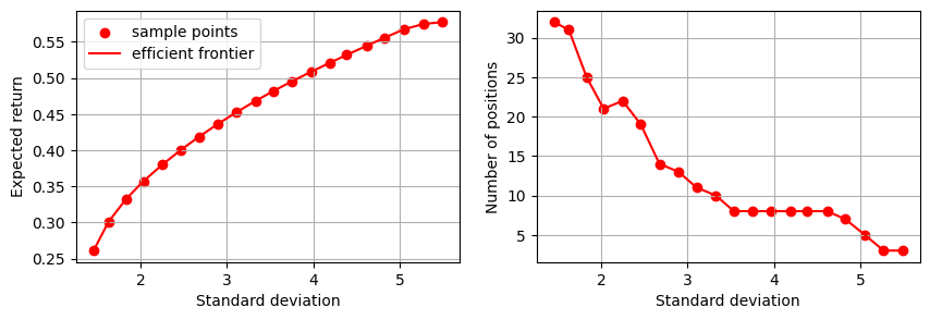
As expected, the number of open positions decreases as we allow more variance; the optimization will progressively invest in fewer high-risk but high-yield assets.