Note
Download this Jupyter notebook and all
data
(unzip next to the ipynb file!).
You will need a Gurobi license to run this notebook, please follow the
license instructions.
Maximizing Return
The standard mean-variance (Markowitz) portfolio selection model determines an optimal investment portfolio that balances risk and expected return. In this notebook, we maximize the expected return of the portfolio while constraining the admissible variance (risk) to a given maximum level. Please refer to the annotated list of references for more background information on portfolio optimization.
[2]:
import gurobipy as gp
import pandas as pd
import numpy as np
import matplotlib.pyplot as plt
Input Data
The following input data is used within the model:
\(S\): set of stocks
\(\mu\): vector of expected returns
\(\Sigma\): PSD variance-covariance matrix
\(\sigma_{ij}\) covariance between returns of assets \(i\) and \(j\)
\(\sigma_{ii}\) variance of return of asset \(i\)
[4]:
# Import example data
Sigma = pd.read_pickle("sigma.pkl")
mu = pd.read_pickle("mu.pkl")
Formulation
The model maximizes the overall expected return for a prespecified maximum level of variance (risk). Mathematically, this results in a convex quadratically constrained optimization problem.
Decision Variables and Variable Bounds
The decision variables in the model are the proportions of capital invested among the considered stocks. The corresponding vector of positions is denoted by \(x\) with its component \(x_i\) denoting the proportion of capital invested in stock \(i\).
Each position must be between 0 and 1; this prevents leverage and short-selling:
Constraints
The budget constraint ensures that all capital is invested:
The estimated risk must not exceed a prespecified maximal admissible level of variance \(\bar\sigma^2\):
Objective Function
The objective is to maximize the expected return of the portfolio:
Using gurobipy, this can be expressed as follows:
[5]:
V = 3.5  # maximal admissible variance (sigma^2)

# Create an empty optimization model
m = gp.Model()

# Add variables: x[i] denotes the proportion invested in stock i
# 0 <= x[i] <= 1
x = m.addMVar(len(mu), lb=0, ub=1, name="x")

# Budget constraint: all investments sum up to 1
m.addConstr(x.sum() == 1, name="Budget_Constraint")

# Limit on variance
risk_constr = m.addConstr(x @ Sigma.to_numpy() @ x <= V, name="Variance")

# Define objective function: Maximize expected return
m.setObjective(mu.to_numpy() @ x, gp.GRB.MAXIMIZE)
We now solve the optimization problem:
[6]:
m.optimize()
Gurobi Optimizer version 13.0.2 build v13.0.2rc1 (linux64 - "Ubuntu 24.04.4 LTS")

CPU model: AMD EPYC 7763 64-Core Processor, instruction set [SSE2|AVX|AVX2]
Thread count: 1 physical cores, 2 logical processors, using up to 2 threads

WLS license 2443533 - registered to Gurobi GmbH
Optimize a model with 1 rows, 462 columns and 462 nonzeros (Max)
Model fingerprint: 0x1ba1fb96
Model has 462 linear objective coefficients
Model has 1 quadratic constraint
Coefficient statistics:
  Matrix range     [1e+00, 1e+00]
  QMatrix range    [3e-03, 1e+02]
  Objective range  [7e-02, 6e-01]
  Bounds range     [1e+00, 1e+00]
  RHS range        [1e+00, 1e+00]
  QRHS range       [4e+00, 4e+00]

Presolve time: 0.04s
Presolved: 463 rows, 925 columns, 107877 nonzeros
Presolved model has 1 second-order cone constraint
Ordering time: 0.01s

Barrier statistics:
 AA' NZ     : 1.070e+05
 Factor NZ  : 1.074e+05 (roughly 1 MB of memory)
 Factor Ops : 3.319e+07 (less than 1 second per iteration)
 Threads    : 1

                  Objective                Residual
Iter       Primal          Dual         Primal    Dual     Compl     Time
   0   1.60528172e+01  1.30801027e+00  6.81e+01 5.81e-02  3.11e-02     0s
   1   1.83483549e+00  1.18107227e+00  6.55e+00 6.39e-08  3.45e-03     0s
   2   3.57409004e-01  6.75808545e-01  4.56e-01 7.03e-14  4.56e-04     0s
   3   2.59566117e-01  4.27509262e-01  5.02e-07 1.78e-14  1.21e-04     0s
   4   3.01938754e-01  3.89407311e-01  9.85e-08 1.21e-14  6.30e-05     0s
   5   3.22233281e-01  3.53419563e-01  1.14e-09 2.73e-15  2.25e-05     0s
   6   3.35242668e-01  3.45815179e-01  1.02e-12 1.67e-16  7.62e-06     0s
   7   3.36987652e-01  3.39306375e-01  6.77e-13 2.78e-17  1.67e-06     0s
   8   3.37616442e-01  3.37940086e-01  1.22e-12 1.11e-16  2.33e-07     0s
   9   3.37760532e-01  3.37790030e-01  6.47e-12 2.22e-16  2.13e-08     0s
  10   3.37772306e-01  3.37773658e-01  3.24e-13 2.22e-16  9.74e-10     0s
  11   3.37773461e-01  3.37773559e-01  2.76e-12 1.50e-15  7.08e-11     0s

Barrier solved model in 11 iterations and 0.29 seconds (0.70 work units)
Optimal objective 3.37773461e-01
Display basic solution data:
[7]:
print(f"Expected return:  {m.ObjVal:.6f}")
print(f"Variance:         {x.X @ Sigma @ x.X:.6f}")
print(f"Solution time:    {m.Runtime:.2f} seconds\n")

# Print investments (with non-negligible values, i.e., > 1e-5)
positions = pd.Series(name="Position", data=x.X, index=mu.index)
print(f"Number of trades: {positions[positions > 1e-5].count()}\n")
print(positions[positions > 1e-5])
Expected return:  0.337773
Variance:         3.500000
Solution time:    0.30 seconds

Number of trades: 25

TSLA    0.007043
KR      0.042551
PGR     0.126962
ORLY    0.048961
ODFL    0.032509
MNST    0.007623
KDP     0.081957
META    0.012825
UNH     0.017630
AVGO    0.048820
DXCM    0.012487
NFLX    0.015324
LLY     0.229237
DPZ     0.039873
MKTX    0.004651
WST     0.024255
TMUS    0.044873
NOC     0.048752
MOH     0.003094
MSFT    0.016649
WM      0.008720
TTWO    0.038637
ENPH    0.005492
NVDA    0.080907
AZO     0.000168
Name: Position, dtype: float64
Efficient Frontier
The efficient frontier reveals the balance between risk and return in investment portfolios. It shows the best-expected return level that can be achieved for a specified risk level. We compute this by solving the above optimization problem for a sample of admissible risk levels.
[8]:
risks = np.linspace(1.37, 4, 20)
returns = np.zeros(risks.shape)
npos = np.zeros(risks.shape)

# hide Gurobi log output
m.params.OutputFlag = 0

# solve the model for each risk level
for i, risk_level in enumerate(risks):
    # set risk level: RHS of risk constraint
    risk_constr.QCRHS = risk_level**2
    m.optimize()
    # store data
    returns[i] = mu @ x.X
    npos[i] = len(x.X[x.X > 1e-5])
Next, we display the efficient frontier for this model: We plot the expected returns (on the \(y\)-axis) against the standard deviation \(\sqrt{x^\top\Sigma x}\) of the expected returns (on the \(x\)-axis). We also display the relationship between the risk and the number of positions in the optimal portfolio.
[9]:
fig, axs = plt.subplots(1, 2, figsize=(10, 3))

# Axis 0: The efficient frontier
axs[0].scatter(x=risks, y=returns, marker="o", label="sample points", color="Red")
axs[0].plot(risks, returns, label="efficient frontier", color="Red")
axs[0].set_xlabel("Standard deviation")
axs[0].set_ylabel("Expected return")
axs[0].legend()
axs[0].grid()

# Axis 1: The number of open positions
axs[1].scatter(x=risks, y=npos, color="Red")
axs[1].plot(risks, npos, color="Red")
axs[1].set_xlabel("Standard deviation")
axs[1].set_ylabel("Number of positions")
axs[1].grid()

plt.show()
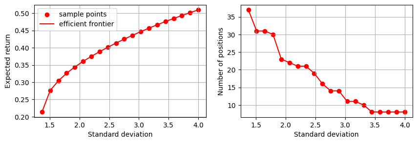
As expected, the number of open positions decreases as we allow more variance; the optimization will progressively invest in fewer high-risk but high-yield assets.