Note
Download this Jupyter notebook and all
data
(unzip next to the ipynb file!).
You will need a Gurobi license to run this notebook, please follow the
license instructions.
Cardinality Constraints
The standard mean-variance (Markowitz) portfolio selection model determines an optimal investment portfolio that balances risk and expected return. In this notebook, we minimize the variance (risk) of the portfolio, constraining the expected return to meet a prescribed minimum level. Please refer to the annotated list of references for more background information on portfolio optimization.
To this basic model, we add cardinality constraints to
limit the number of open positions and
limit the minimum size of each position.
These limits are often used to reduce transaction costs and simplify the rebalancing and management of the portfolio.
[2]:
import gurobipy as gp
import pandas as pd
import numpy as np
import matplotlib.pyplot as plt
Input Data
The following input data is used within the model:
\(S\): set of stocks
\(\mu\): vector of expected returns
\(\Sigma\): PSD variance-covariance matrix
\(\sigma_{ij}\) covariance between returns of assets \(i\) and \(j\)
\(\sigma_{ii}\) variance of return of asset \(i\)
[4]:
# Import some example data set
Sigma = pd.read_pickle("sigma.pkl")
mu = pd.read_pickle("mu.pkl")
Formulation
The model minimizes the variance of the portfolio given that the minimum level of expected return is attained, that the number of positions held does not exceed a specified number, and that the size of each position does not fall below a certain level.
Mathematically, this results in a convex quadratic mixed-integer optimization problem.
Model Parameters
We use the following parameters:
\(\bar\mu\): required expected portfolio return
\(K\): maximal number of stocks in the portfolio
\(\ell>0\): lower bound on position size
[5]:
# Values for the model parameters:
r = 0.25  # Required return
K = 15  # Maximal number of stocks
l = 0.00001  # Minimal position size
Decision Variables
We need two sets of decision variables:
The proportions of capital invested among the considered stocks. The corresponding vector of positions is denoted by \(x\) with its component \(x_i\) denoting the proportion of capital invested in stock \(i\).
Binary variables \(b_i\) indicating whether or not asset \(i\) is held. If \(b_i\) is 0, the holding \(x_i\) is also 0; otherwise if \(b_i\) is 1, the investor holds asset \(i\) (that is, \(x_i \geq \ell\)).
Variable Bounds
Each position must be between 0 and 1; this prevents leverage and short-selling:
The \(b_i\) must be binary:
[6]:
%%capture
# Create an empty optimization model
m = gp.Model()

# Add variables: x[i] denotes the proportion invested in stock i
x = m.addMVar(len(mu), lb=0, ub=1, name="x")

# Add variables: b[i]=1 if stock i is held, and b[i]=0 otherwise
b = m.addMVar(len(mu), vtype=gp.GRB.BINARY, name="b")
Constraints
The budget constraint ensures that all capital is invested:
The expected return of the portfolio must be at least \(\bar\mu\):
The variable bounds only enforce that each \(x_i\) is between \(0\) and \(1\). To enforce the minimal position size, we use the binary variables \(b\) and the following sets of discrete constraints:
Ensure that \(x_i = 0\) if \(b_i = 0\):
\begin{equation*} x_i \leq b_i \; , \; i \in S\tag{1} \end{equation*}
Note that \(x_i\) has an upper bound of 1. Thus, if \(b_i = 1\), the above constraint is non-restrictive.
Ensure a minimal position size of \(\ell\) if asset \(i\) is traded:
\begin{equation*} x_i \geq \ell b_i \; , \; i \in S\tag{2} \end{equation*}
Hence \(b_i = 1\) implies \(x_i \geq \ell\). If \(b_i = 0\), this constraint is non-restrictive since \(x_i\) has a lower bound of 0.
Finally, there must be at most \(K\) positions in the portfolio:
\begin{equation*} \sum_{i \in S} b_i \leq K \end{equation*}
[7]:
# Budget constraint: all investments sum up to 1
m.addConstr(x.sum() == 1, "Budget_Constraint")

# Lower bound on expected return
m.addConstr(mu.to_numpy() @ x >= r, "Minimal_Return")

# Force x to 0 if not traded; see formula (1) above
m.addConstr(x <= b, name="Indicator")

# Minimal position; see formula (2) above
m.addConstr(x >= l * b, name="Minimal_Position")

# Cardinality constraint: at most K positions
cardinality_constr = m.addConstr(b.sum() <= K, "Cardinality")
Objective Function
The objective is to minimize the risk of the portfolio, which is measured by its variance:
[8]:
# Define objective function: Minimize risk
m.setObjective(x @ Sigma.to_numpy() @ x, gp.GRB.MINIMIZE)
We now solve the optimization problem:
[9]:
m.optimize()
Gurobi Optimizer version 13.0.2 build v13.0.2rc1 (linux64 - "Ubuntu 24.04.4 LTS")

CPU model: AMD EPYC 7763 64-Core Processor, instruction set [SSE2|AVX|AVX2]
Thread count: 1 physical cores, 2 logical processors, using up to 2 threads

WLS license 2443533 - registered to Gurobi GmbH
Optimize a model with 927 rows, 924 columns and 3234 nonzeros (Min)
Model fingerprint: 0x73f3de97
Model has 0 linear objective coefficients
Model has 106953 quadratic objective terms
Variable types: 462 continuous, 462 integer (462 binary)
Coefficient statistics:
  Matrix range     [1e-05, 1e+00]
  Objective range  [0e+00, 0e+00]
  QObjective range [6e-03, 2e+02]
  Bounds range     [1e+00, 1e+00]
  RHS range        [2e-01, 2e+01]

Found heuristic solution: objective 21.1318982
Presolve time: 0.05s
Presolved: 927 rows, 924 columns, 3233 nonzeros
Presolved model has 106953 quadratic objective terms
Variable types: 462 continuous, 462 integer (462 binary)

Root relaxation: objective 2.026597e+00, 154 iterations, 0.01 seconds (0.01 work units)

    Nodes    |    Current Node    |     Objective Bounds      |     Work
 Expl Unexpl |  Obj  Depth IntInf | Incumbent    BestBd   Gap | It/Node Time

     0     0    2.02660    0   37   21.13190    2.02660  90.4%     -    0s
H    0     0                       2.5684442    2.02660  21.1%     -    0s
H    0     0                       2.1483555    2.02660  5.67%     -    0s
H    0     0                       2.1373929    2.02660  5.18%     -    0s
H    0     0                       2.1316137    2.02660  4.93%     -    0s
     0     0    2.02660    0   37    2.13161    2.02660  4.93%     -    0s
     0     0    2.02660    0   38    2.13161    2.02660  4.93%     -    0s
     0     0    2.02660    0   37    2.13161    2.02660  4.93%     -    0s
     0     0    2.02660    0   38    2.13161    2.02660  4.93%     -    0s
     0     0    2.02660    0   38    2.13161    2.02660  4.93%     -    0s
H    0     0                       2.0970867    2.02660  3.36%     -    0s
H    0     0                       2.0943481    2.02660  3.23%     -    0s
H    0     0                       2.0685556    2.02660  2.03%     -    0s
H    0     0                       2.0661170    2.02660  1.91%     -    0s
     0     1    2.02660    0   38    2.06612    2.02660  1.91%     -    0s
  5151   941    2.05987   32   22    2.06612    2.04693  0.93%   4.3    5s
 11717  1162    2.06450   29   22    2.06612    2.05554  0.51%   4.0   10s
 17855   691     cutoff   21         2.06612    2.06094  0.25%   4.0   15s

Cutting planes:
  MIR: 5
  Flow cover: 3

Explored 20386 nodes (82003 simplex iterations) in 16.61 seconds (25.83 work units)
Thread count was 2 (of 2 available processors)

Solution count 9: 2.06612 2.06856 2.09435 ... 21.1319

Optimal solution found (tolerance 1.00e-04)
Best objective 2.066116973868e+00, best bound 2.065910672679e+00, gap 0.0100%
Display basic solution data:
[10]:
print(f"Minimum Risk:     {m.ObjVal:.6f}")
print(f"Expected return:  {mu @ x.X:.6f}")
print(f"Solution time:    {m.Runtime:.2f} seconds\n")
print(f"Number of trades: {sum(b.X)}\n")

# Print investments (with non-negligible value, i.e. >1e-5)
positions = pd.Series(name="Position", data=x.X, index=mu.index)
print(positions[positions > 1e-5])
Minimum Risk:     2.066117
Expected return:  0.250000
Solution time:    16.62 seconds

Number of trades: 15.0

KR      0.040359
PGR     0.051136
CME     0.049374
ODFL    0.044432
KDP     0.087797
CLX     0.073365
SJM     0.060471
LLY     0.104751
DPZ     0.058761
MRK     0.073922
ED      0.110132
TMUS    0.047234
WM      0.073017
TTWO    0.047324
WMT     0.077925
Name: Position, dtype: float64
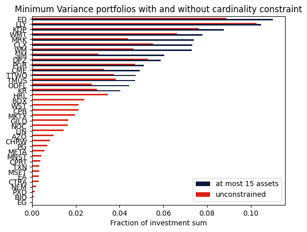
Comparison with the unconstrained portfolio
We can also compute the portfolio without the cardinality constraint and compare the resulting portfolios.
[11]:
# remove cardinality constraint
m.remove(cardinality_constr)
m.params.OutputFlag = 0
m.optimize()

# retrieve and display solution data
positions_unconstr = pd.Series(name="Position", data=x.X, index=mu.index)
mask = (positions > 1e-5) | (positions_unconstr > 1e-5)
df = pd.DataFrame(
    index=positions[mask].index,
    data={
        "at most 15 assets": positions,
        "unconstrained": positions_unconstr,
    },
).sort_values(by=["at most 15 assets", "unconstrained"], ascending=True)

axs = df.plot.barh(color=["#0b1a3c", "#dd2113"])
axs.set_xlabel("Fraction of investment sum")
plt.title("Minimum Variance portfolios with and without cardinality constraint")
plt.show()
Takeaways
Cardinality constraints can be modeled using binary decision variables.
This already leads to non-trivial combinatorial optimization problems, which can be solved using Gurobi.