Note
Download this Jupyter notebook and all
data
(unzip next to the ipynb file!).
You will need a Gurobi license to run this notebook, please follow the
license instructions.
Rebalancing with Transaction Costs
The standard mean-variance (Markowitz) portfolio selection model determines an optimal investment portfolio that balances risk and expected return. Please refer to the annotated list of references for more background information on portfolio optimization.
In this notebook, we rebalance an existing portfolio to maximize the expected return of the portfolio while constraining the admissible variance (risk) to a given maximum level. Additionally, we account for transaction costs and fees:
The fixed transaction costs occur for each transaction and are independent of the amount that is bought or sold.
The variable transaction fees are proportional to the traded amount.
[2]:
import gurobipy as gp
import pandas as pd
import numpy as np
import random
import matplotlib.pyplot as plt
Input Data
The following input data is used within the model:
\(S\): set of stocks
\(\mu\): vector of expected returns
\(\Sigma\): PSD variance-covariance matrix
\(\sigma_{ij}\) covariance between returns of assets \(i\) and \(j\)
\(\sigma_{ii}\) variance of return of asset \(i\)
[4]:
# Import some example data set
Sigma = pd.read_pickle("sigma.pkl")
mu = pd.read_pickle("mu.pkl")
Formulation
The model rebalances an existing portfolio. It maximizes the expected return of the new portfolio, constraining the variance of the portfolio not to exceed a specified level, and also accounts for fixed and variable transaction costs and fees. Mathematically, this results in a convex quadratically constrained mixed-integer optimization problem.
Model parameters
The following parameters are used within the model:
\(\bar\sigma^2\): maximal admissible variance for the portfolio return
\(x^0_i\): holdings of asset \(i\) in the initial portfolio. Usually, the starting portfolio is given by the previous trading period. In this notebook, we choose a simple starting portfolio by equally distributing the capital among the assets with the largest returns.
\(\ell>0\): lower bound on transaction size
\(c_i^+, c_i^-\): fixed transaction cost when buying/selling stock \(i\)
\(f_i^+, f_i^-\): variable transaction cost for buying/selling stock \(i\), relative to total investment value
[5]:
# Values for the model parameters:
V = 4.0  # Maximal admissible variance (sigma^2)
l = 0.001  # Minimal transaction size

# Fixed transaction costs
c_plus = 0.00002 * np.ones(mu.shape)
c_minus = 0.00002 * np.ones(mu.shape)
# Variable transaction fees
f_plus = 0.0002 * np.ones(mu.shape)
f_minus = 0.0002 * np.ones(mu.shape)

# Initial portfolio:  Equally distributed among largest return assets
x0 = pd.Series(index=mu.index, data=np.zeros(mu.shape))
x0.loc[mu.nlargest(20).index] = 1.0 / 20.0
Decision Variables
We need several sets of decision variables:
The proportions of capital invested in the rebalanced portfolio among the considered stocks. The corresponding vector of positions is denoted by \(x\) with its component \(x_i\) denoting the proportion of capital invested in stock \(i\).
The other sets of variables distinguish between buys and sells:
The proportions of each stock bought and included in the rebalanced portfolio. The corresponding vector of positions is denoted by \(x^+\) with its component \(x^+_i\) denoting the proportion of capital representing the purchase of stock \(i\).
The proportions of each stock sold from the existing portfolio. The corresponding vector of sales is denoted by \(x^-\) with its component \(x^-_i\) denoting the proportion of capital representing the sale of stock \(i\).
Binary variables \(b_i^+\) indicating whether or not asset \(i\) is bought. If \(b_i^+\) is 0, asset \(i\) is not bought, that is \(x_i \leq x^0_i\). Otherwise, if \(b_i^+\) is 1, the investor buys some amount (at least \(\ell\)) of asset \(i\) and \(x_i \geq x^0_i + \ell\).
Binary variables \(b_i^-\) indicating whether or not asset \(i\) is sold. If \(b_i^-\) is 0, asset \(i\) is not sold, that is \(x_i \geq x^0_i\). Otherwise, if \(b_i^-\) is 1, the investor sells some amount (at least \(\ell\)) of asset \(i\) and \(x_i \leq x^0_i - \ell\).
Variable Bounds
Each position must be between 0 and 1; this prevents leverage and short-selling:
The buy and sell proportions must be non-negative:
Variables \(b_i^+, b_i^-\) are binary:
[6]:
# Create an empty optimization model
m = gp.Model()

# Add variables: x[i] denotes the proportion invested in stock i
x = m.addMVar(len(mu), lb=0, ub=1, name="x")
# Add variables: x_plus[i] denotes the proportion of stock i bought
x_plus = m.addMVar(len(mu), lb=0, ub=1, name="x_plus")
# Add variables: x_minus[i] denotes the proportion of stock i sold
x_minus = m.addMVar(len(mu), lb=0, ub=1, name="x_minus")
# Add variables: b_plus[i]=1 if stock i is bought, and b_plus[i]=0 otherwise
b_plus = m.addMVar(len(mu), vtype=gp.GRB.BINARY, name="b_plus")
# Add variables: b_minus[i]=1 if stock i is sold, and b_minus[i]=0 otherwise
b_minus = m.addMVar(len(mu), vtype=gp.GRB.BINARY, name="b_minus")
Constraints
The final proportion of capital invested in a stock in the rebalanced portfolio is obtained by taking into account the buys and sells of this stock as well as the initial holdings in the existing portfolio:
\begin{equation*} x_i = x^0_i + x^+_i - x^-_i \; , \; i \in S \tag{1} \end{equation*}
The estimated risk must not exceed a prespecified maximal admissible level of variance \(\bar\sigma^2\):
[7]:
%%capture
# Proportion Changes balance constraint; see formula (1) above
m.addConstr(x == x0.to_numpy() + x_plus - x_minus, name="Position_Balance")

# Upper bound on variance
m.addConstr(x @ Sigma.to_numpy() @ x <= V, name="Variance")
Note that in an optimal solution, at most one of the two variables \(x^+_i\) and \(x^-_i\) should take a nonzero value for each \(i\).
To enforce the minimal transaction size, we use the binary variables \(b^+,b^-\) and the following sets of discrete constraints, which will enforce:
\begin{equation*} x_i^+ \geq \ell\ \text{ if } b_i^+=1 \ \text{ and } x_i^+ = 0 \text{ otherwise} \\ \end{equation*} \begin{equation*} x_i^- \geq \ell\ \text{ if } b_i^-=1 \ \text{ and } x_i^- = 0 \text{ otherwise} \end{equation*}
Ensure that \(x_i^+ = 0\) if \(b_i^+ = 0\):
\begin{equation*} x_i^+ \leq b_i^+ \; , \; i \in S\tag{2} \end{equation*}
Note that we are using that \(x_i^+\) has an upper bound of 1 because we cannot buy or sell more than the total capital in one position. Hence, if \(b_i^+ = 1\), the above constraint is non-restrictive.
Ensure a minimal transaction size of \(\ell\) if asset \(i\) is traded:
\begin{equation*} x_i^+ \geq \ell b_i^+ \; , \; i \in S\tag{3} \end{equation*}
Hence \(b_i^+ = 1\) implies \(x_i^+ \geq \ell\). If \(b_i^+ = 0\), this constraint is non-restrictive since \(x_i^+\) has a lower bound of 0.
Analogously, we define similar constraints for \(x_i^-\) and \(b_i^-\):
Finally, we require that the same asset is not bought and sold at the same time:
[8]:
%%capture
# Force x_plus, x_minus to 0 if not traded; see formula (2) above
m.addConstr(x_plus <= b_plus, name="Indicator_Buy")
m.addConstr(x_minus <= b_minus, name="Indicator_Sell")
# Minimal buy/sell; see formula (3) above
m.addConstr(x_plus >= l * b_plus, name="Minimal_Buy")
m.addConstr(x_minus >= l * b_minus, name="Minimal_Sell")

# Constraint preventing the simultaneous buy and sell of the same security
m.addConstr(b_plus + b_minus <= 1, name="Mutual_Exclusivity")
Without any costs and fees, we would have the budget constraint \(\sum_{i} x_i = 1\) to ensure that all investments sum up to one. However, we must also pay the resulting fixed costs and variable transaction fees from the capital.
The fixed costs occur once per transaction (purchase or sale) and do not depend on the transaction size; hence the fixed costs for asset \(i\) are \(c_i^+b_i^+ + c_i^-b_i^-\). The variable fees are proportional to the transaction size; hence the fees for asset \(i\) are \(f_i^+x_i^+ + f_i^-x_i^-\).
We include these in the the left-hand side of the equation:
\begin{equation*} \underbrace{\sum_{i \in S}x_i}_\text{investments} + \underbrace{\sum_{i \in S}c_i^+b_i^+ + \sum_{i\in S}c_i^-b_i^-}_\text{fixed costs for buying and selling} + \underbrace{\sum_{i \in S}f_i^+x_i^+ + \sum_{i \in S}f_i^-x_i^-}_\text{variable fees for buying and selling} = 1 \tag{4} \end{equation*}
[9]:
# Budget constraint: all investments, costs, and fees sum up to 1, see formula (4) above
budget_constr = m.addConstr(
    x.sum() + c_plus @ b_plus + c_minus @ b_minus + f_plus @ x_plus + f_minus @ x_minus
    == 1,
    name="Budget_Constraint",
)
Objective Function
The objective is to maximize the expected return of the portfolio:
[10]:
# Define objective: Maximize expected return
m.setObjective(mu.to_numpy() @ x, gp.GRB.MAXIMIZE)
We now solve the optimization problem to provable optimality of 1%. By default, Gurobi uses a MIP gap of 1e-4 (=0.01%), but many real-world application do not need such a tight gap. Hence, we relax this to 1% to improve performance.
[11]:
m.Params.MIPGap = 0.01
m.optimize()
Set parameter MIPGap to value 0.01
Gurobi Optimizer version 13.0.2 build v13.0.2rc1 (linux64 - "Ubuntu 24.04.4 LTS")

CPU model: AMD EPYC 7763 64-Core Processor, instruction set [SSE2|AVX|AVX2]
Thread count: 1 physical cores, 2 logical processors, using up to 2 threads

Non-default parameters:
MIPGap  0.01

WLS license 2443533 - registered to Gurobi GmbH
Optimize a model with 2773 rows, 2310 columns and 8316 nonzeros (Max)
Model fingerprint: 0xa5e8a251
Model has 462 linear objective coefficients
Model has 1 quadratic constraint
Variable types: 1386 continuous, 924 integer (924 binary)
Coefficient statistics:
  Matrix range     [2e-05, 1e+00]
  QMatrix range    [3e-03, 1e+02]
  Objective range  [7e-02, 6e-01]
  Bounds range     [1e+00, 1e+00]
  RHS range        [5e-02, 1e+00]
  QRHS range       [4e+00, 4e+00]

Presolve removed 1788 rows and 1346 columns
Presolve time: 0.13s
Presolved: 985 rows, 964 columns, 2972 nonzeros
Presolved model has 1 quadratic constraint(s)
Variable types: 482 continuous, 482 integer (482 binary)

Root relaxation: objective 5.916849e-01, 39 iterations, 0.00 seconds (0.00 work units)

    Nodes    |    Current Node    |     Objective Bounds      |     Work
 Expl Unexpl |  Obj  Depth IntInf | Incumbent    BestBd   Gap | It/Node Time

     0     0    0.59168    0    1          -    0.59168      -     -    0s
     0     0    0.56263    0    2          -    0.56263      -     -    0s
H    0     0                       0.2876866    0.56262  95.6%     -    1s
H    0     0                       0.2975177    0.56262  89.1%     -    1s
H    0     0                       0.2980427    0.56262  88.8%     -    1s
H    0     0                       0.2983194    0.56262  88.6%     -    1s
H    0     0                       0.2983239    0.56262  88.6%     -    1s
H    0     0                       0.2983538    0.56262  88.6%     -    1s
H    0     0                       0.2983548    0.56262  88.6%     -    1s
     0     0    0.43881    0    3    0.29835    0.43881  47.1%     -    1s
     0     0    0.43876    0    4    0.29835    0.43876  47.1%     -    1s
     0     0    0.42962    0    4    0.29835    0.42962  44.0%     -    2s
     0     0    0.42883    0    5    0.29835    0.42883  43.7%     -    2s
     0     0    0.41341    0    6    0.29835    0.41341  38.6%     -    2s
     0     0    0.41341    0    6    0.29835    0.41341  38.6%     -    2s
     0     0    0.40037    0    5    0.29835    0.40037  34.2%     -    2s
     0     0    0.39494    0    5    0.29835    0.39494  32.4%     -    2s
     0     0    0.39260    0    7    0.29835    0.39260  31.6%     -    2s
     0     0    0.39260    0    6    0.29835    0.39260  31.6%     -    2s
     0     0    0.39238    0    7    0.29835    0.39238  31.5%     -    2s
     0     0    0.38959    0    7    0.29835    0.38959  30.6%     -    2s
     0     0    0.38905    0    9    0.29835    0.38905  30.4%     -    2s
     0     0    0.38818    0    9    0.29835    0.38818  30.1%     -    2s
     0     0    0.38471    0    8    0.29835    0.38471  28.9%     -    3s
     0     0    0.37920    0    7    0.29835    0.37920  27.1%     -    3s
     0     0    0.37838    0    6    0.29835    0.37838  26.8%     -    3s
     0     0    0.37776    0    8    0.29835    0.37776  26.6%     -    3s
     0     0    0.37755    0    8    0.29835    0.37755  26.5%     -    3s
     0     0    0.37675    0    8    0.29835    0.37675  26.3%     -    3s
     0     0    0.37633    0    8    0.29835    0.37633  26.1%     -    3s
     0     0    0.37633    0    8    0.29835    0.37633  26.1%     -    3s
     0     0    0.37633    0    8    0.29835    0.37633  26.1%     -    3s
H    0     0                       0.3299732    0.37633  14.0%     -    4s
H    0     0                       0.3347700    0.37633  12.4%     -    4s
     0     2    0.37633    0    8    0.33477    0.37633  12.4%     -    5s
H   17    17                       0.3434110    0.37632  9.58%   2.8    5s
H   22    22                       0.3467035    0.37632  8.54%   3.5    5s
H   38    38                       0.3477116    0.37631  8.22%   4.3    5s
H   52    52                       0.3477161    0.37625  8.21%   5.6    6s
H   52    52                       0.3477194    0.37625  8.21%   5.6    6s
H   52    52                       0.3477614    0.37625  8.19%   5.6    6s
H   52    52                       0.3483063    0.37625  8.02%   5.6    6s
H   54    54                       0.3483120    0.37625  8.02%   5.4    6s
H   54    54                       0.3516142    0.37625  7.01%   5.4    6s
H   54    54                       0.3518390    0.37625  6.94%   5.4    6s
H   54    54                       0.3521468    0.37625  6.85%   5.4    6s
H   54    54                       0.3524167    0.37625  6.76%   5.4    6s
H   54    54                       0.3524822    0.37625  6.74%   5.4    7s
H   54    54                       0.3525002    0.37625  6.74%   5.4    7s
H  278   242                       0.3525004    0.35893  1.82%   7.8   10s
H  278   226                       0.3532388    0.35893  1.61%   7.8   10s

Explored 280 nodes (3055 simplex iterations) in 10.98 seconds (11.27 work units)
Thread count was 2 (of 2 available processors)

Solution count 10: 0.353239 0.3525 0.352417 ... 0.347712

Optimal solution found (tolerance 1.00e-02)
Best objective 3.532388437286e-01, best bound 3.538516402191e-01, gap 0.1735%
Display basic solution data, costs, and fees. For clarity, we round all solution quantities to five digits.
[12]:
print(f"Expected return:  {m.ObjVal:.6f}")
print(f"Variance:         {x.X @ Sigma @ x.X:.6f}")
print(f"Solution time:    {m.Runtime:.2f} seconds\n")
print(f"Fixed costs:      {c_plus @ b_plus.X + c_minus @ b_minus.X:.6f}")
print(f"Variable fees:    {f_plus @ x_plus.X + f_minus @ x_minus.X:.6f}\n")
print(
    f"Number of positions: before {np.count_nonzero(x0[x0>1e-5])}, after {np.count_nonzero(x.X[x.X>1e-5])}"
)
print(
    f"Number of trades:    {sum(b_plus.X.round()) + sum(b_minus.X.round())} ({sum(b_plus.X.round())} buy(s), {sum(b_minus.X.round())} sell(s))\n"
)

# Print all assets with either a non-negligible position or transaction
df = pd.DataFrame(
    index=mu.index,
    data={
        "position": x.X,
        "transaction": x_plus.X - x_minus.X,
    },
).round(6)
df[(df["position"] > 1e-5) | (abs(df["transaction"]) > 1e-5)].sort_values(
    "position", ascending=False
)
Expected return:  0.353239
Variance:         3.999998
Solution time:    10.99 seconds

Fixed costs:      0.000620
Variable fees:    0.000330

Number of positions: before 20, after 19
Number of trades:    31.0 (13.0 buy(s), 18.0 sell(s))
[12]:
| position | transaction | |
|---|---|---|
| LLY | 0.251090 | 0.251090 |
| PGR | 0.129798 | 0.129798 |
| NVDA | 0.108950 | 0.058950 |
| KDP | 0.066010 | 0.066010 |
| ORLY | 0.053971 | 0.053971 |
| NOC | 0.052205 | 0.052205 |
| AVGO | 0.050000 | 0.000000 |
| TMUS | 0.040526 | 0.040526 |
| ODFL | 0.038888 | 0.038888 |
| TTWO | 0.035145 | 0.035145 |
| DPZ | 0.032106 | 0.032106 |
| KR | 0.030027 | 0.030027 |
| NFLX | 0.021928 | -0.028072 |
| UNH | 0.020223 | 0.020223 |
| DXCM | 0.018073 | -0.031927 |
| TSLA | 0.016058 | -0.033942 |
| META | 0.015302 | 0.015302 |
| ENPH | 0.011035 | -0.038965 |
| MOH | 0.007708 | -0.042292 |
| AMD | 0.000005 | -0.049995 |
| MU | 0.000000 | -0.050000 |
| KLAC | 0.000000 | -0.050000 |
| CDNS | 0.000000 | -0.050000 |
| NOW | 0.000000 | -0.050000 |
| FICO | 0.000000 | -0.050000 |
| AMAT | 0.000000 | -0.050000 |
| MPWR | 0.000000 | -0.050000 |
| AXON | 0.000000 | -0.050000 |
| EPAM | 0.000000 | -0.050000 |
| FANG | 0.000000 | -0.050000 |
| PANW | 0.000000 | -0.050000 |
| LRCX | 0.000000 | -0.050000 |
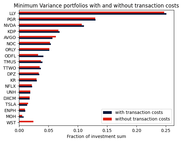
Comparison with the unconstrained portfolio
We can also optimize the portfolio without considering the transaction costs and compare the resulting portfolios.
[13]:
# remove budget constraint
m.remove(budget_constr)
# add new budget constraint without costs
m.addConstr(x.sum() == 1, name="Budget_Constraint")
m.params.OutputFlag = 0
m.optimize()

# retrieve and display solution data
positions_no_costs = pd.Series(name="Position", data=x.X, index=mu.index)
mask = (df["position"] > 1e-5) | (positions_no_costs > 1e-5)
df2 = pd.DataFrame(
    index=df[mask].index,
    data={
        "with transaction costs": df["position"],
        "without transaction costs": positions_no_costs,
    },
).sort_values("with transaction costs", ascending=True)

axs = df2.plot.barh(color=["#0b1a3c", "#dd2113"])
axs.set_xlabel("Fraction of investment sum")
plt.title("Minimum Variance portfolios with and without transaction costs")
plt.show()
Takeaways
Rebalancing is modeled in the same way as when we start from an all-cash position by considering the difference between the initial holdings and the final position in the rebalanced portfolio instead of just the final position.
When rebalancing, we can also sell positions; when starting from an all-cash position, we can only buy (unless we allow short-selling). We introduced additional decision variables for this.
Transaction costs and fees can be incorporated into the basic budget constraint.
Fixed costs are independent of the traded amount and can be modeled using binary decision variables.
Variable fees are proportional to the traded amount and can be modeled using continuous decision variables.