Note
Download this Jupyter notebook and all
data
(unzip next to the ipynb file!).
You will need a Gurobi license to run this notebook, please follow the
license instructions.
Buying Round Lots
The standard mean-variance (Markowitz) portfolio selection model determines the optimal investments by balancing risk and expected return. In this notebook, we minimize the variance (risk) of the portfolio given that the prescribed level of expected return is attained. Please refer to the annotated list of references for more background information on portfolio optimization.
Securities on the stock market are often traded in round lots. A round lot is a fixed number of units (that typically depends on the financial instrument that is traded). For example, stocks are often traded in multiples of 100 shares. Any smaller quantity of traded securities is called an odd lot, which typically induces higher transaction costs, or slower order execution. Also, to avoid small positions, one might want to ensure that a minimum number of units is traded if a position is opened.
In this notebook, we add the following constraints to the basic model:
If a position is opened, it must comprise a minimum number of shares and,
stocks can only be bought in round lots.
For our example, we will be using a lower bound of 1000 shares per asset and a uniform lot size of 100 shares.
We also include a risk-free asset in the model.
[2]:
import gurobipy as gp
import gurobipy_pandas as gppd
import pandas as pd
import numpy as np
import matplotlib.pyplot as plt
Input Data
The following input data is used within the model:
\(S\): set of stocks
\(p_i\): last price of stock \(i\) in USD
\(\mu\): vector of expected returns
\(\Sigma\): PSD variance-covariance matrix
\(\sigma_{ij}\) covariance between returns of assets \(i\) and \(j\)
\(\sigma_{ii}\) variance of return of asset \(i\)
[4]:
# Import some example data set
Sigma = pd.read_pickle("sigma.pkl")
mu = pd.read_pickle("mu.pkl")
We also import the prices of the assets:
[5]:
# Import price data
prices = pd.read_pickle("subset_weekly_closings_10yrs.pkl").tail(1).squeeze()
data = pd.DataFrame(data={"Price": prices})
Formulation
The model minimizes the variance of the portfolio given that the minimum level of expected return is attained. Also
shares can only be bought in multiples of a lot size \(l\), and
if a position in an asset is bought, it must comprise at least \(L\) lots (and hence at least \(L\cdot l\) shares).
Mathematically, this results in a convex quadratic mixed-integer optimization problem.
Model Parameters
We use the following parameters:
\(\bar\mu\): required expected portfolio return
\(\mu_\text{rf}\): risk-free return
\(T\): total investment amount in USD (AUM)
\(L\): minimal number of lots per asset
\(l\): lot size
[6]:
# Values for the model parameters:
r = 0.25  # Required return
mu_rf = 0.5 / 52  # Risk-free return rate
T = 1e7  # total investment amount
L = 10  # minimal number of lots
l = 100  # lot size
Decision Variables
We need three types of decision variables:
The proportions of capital invested among the considered stocks. The corresponding vector of positions is denoted by \(x\) with its component \(x_i\) denoting the proportion of capital invested in stock \(i\).
The proportion of capital invested into the risk-free asset is denoted by \(x_\text{rf}\).
The number of lots of shares bought of the considered stocks. The corresponding vector is denoted by \(z\) with its component \(z_i\) denoting the number of lots in stock \(i\). Note that the number of shares in asset \(i\) is then \(lz_i\).
Variable Bounds
Each position must be between 0 and 1; this prevents leverage and short-selling:
The \(z_i\) must be integers. To enforce the minimal number \(L\) of lots if an asset is bought, we will declare those variables semi-integer. That is,
We will model this using the gurobipy-pandas package. Using this, we first create an extended DataFrame containing the decision variables.
[7]:
# Create an empty optimization model
m = gp.Model()

# Add variable: xrf denotes the proportion of risk-free asset
xrf = m.addVar(lb=0, ub=1, name="x_rf")

# Add variables
df_model = (
    # x[i] denotes the proportion invested in stock i
    data.gppd.add_vars(m, name="x", ub=1)
    # z[i] denotes the number of lots of stock i. Must be integer and greater or equal to L or zero.
    # Defining the variable as semi-integer is enough to enforce the buy-in threshold requirement.
    .gppd.add_vars(m, name="z", vtype=gp.GRB.SEMIINT, lb=L)
)

# Inspect the created DataFrame:
m.update()
df_model
[7]:
| Price | x | z | |
|---|---|---|---|
| APTV | 79.150002 | <gurobi.Var x[APTV]> | <gurobi.Var z[APTV]> |
| DVN | 44.290001 | <gurobi.Var x[DVN]> | <gurobi.Var z[DVN]> |
| HSY | 194.528000 | <gurobi.Var x[HSY]> | <gurobi.Var z[HSY]> |
| CAG | 28.020000 | <gurobi.Var x[CAG]> | <gurobi.Var z[CAG]> |
| HST | 16.980000 | <gurobi.Var x[HST]> | <gurobi.Var z[HST]> |
| ... | ... | ... | ... |
| AEE | 76.779999 | <gurobi.Var x[AEE]> | <gurobi.Var z[AEE]> |
| AAPL | 187.440002 | <gurobi.Var x[AAPL]> | <gurobi.Var z[AAPL]> |
| AIZ | 159.820007 | <gurobi.Var x[AIZ]> | <gurobi.Var z[AIZ]> |
| UNP | 215.690002 | <gurobi.Var x[UNP]> | <gurobi.Var z[UNP]> |
| K | 52.200001 | <gurobi.Var x[K]> | <gurobi.Var z[K]> |
462 rows × 3 columns
Constraints
The budget constraint ensures that the entire capital is invested:
The expected return of the portfolio must be at least \(\bar\mu\):
[8]:
%%capture
# Budget constraint: all investments sum up to 1
m.addConstr(df_model["x"].sum() + xrf == 1, name="Budget_Constraint")

# Lower bound on expected return
m.addConstr(mu.to_numpy() @ df_model["x"] + mu_rf * xrf >= r, "Minimal_Return")
Round lots
The relative position \(x_i\) in stock \(i\) and the number of round lots \(z_i\) are related via the price \(p_i\) as follows:
[9]:
%%capture
gppd.add_constrs(
    m,
    df_model["x"] - l / T * df_model["Price"] * df_model["z"],
    "=",
    0,
    name="match_round_lots",
)
Objective Function
The objective is to minimize the risk of the portfolio, which is measured by its variance:
[10]:
# Define objective function: Minimize risk
m.setObjective(df_model["x"] @ Sigma.to_numpy() @ df_model["x"], gp.GRB.MINIMIZE)
We now solve the optimization problem:
[11]:
m.optimize()
Gurobi Optimizer version 13.0.2 build v13.0.2rc1 (linux64 - "Ubuntu 24.04.4 LTS")

CPU model: AMD EPYC 7763 64-Core Processor, instruction set [SSE2|AVX|AVX2]
Thread count: 1 physical cores, 2 logical processors, using up to 2 threads

WLS license 2443533 - registered to Gurobi GmbH
Optimize a model with 464 rows, 925 columns and 1850 nonzeros (Min)
Model fingerprint: 0x5dd8105c
Model has 0 linear objective coefficients
Model has 106953 quadratic objective terms
Variable types: 463 continuous, 0 integer (0 binary)
Semi-Variable types: 0 continuous, 462 integer
Coefficient statistics:
  Matrix range     [9e-05, 1e+00]
  Objective range  [0e+00, 0e+00]
  QObjective range [6e-03, 2e+02]
  Bounds range     [1e+00, 1e+01]
  RHS range        [2e-01, 1e+00]

Presolve time: 0.02s
Presolved: 1388 rows, 1387 columns, 3697 nonzeros
Presolved model has 106953 quadratic objective terms
Variable types: 463 continuous, 924 integer (462 binary)
Found heuristic solution: objective 11.4196528

Root relaxation: objective 1.803654e+00, 161 iterations, 0.01 seconds (0.01 work units)

    Nodes    |    Current Node    |     Objective Bounds      |     Work
 Expl Unexpl |  Obj  Depth IntInf | Incumbent    BestBd   Gap | It/Node Time

     0     0    1.80365    0   62   11.41965    1.80365  84.2%     -    0s
H    0     0                       2.6779857    1.80365  32.6%     -    0s
H    0     0                       2.6491462    1.80365  31.9%     -    0s
H    0     0                       2.6455642    1.80365  31.8%     -    0s
H    0     0                       2.6443389    1.80365  31.8%     -    0s
H    0     0                       2.0051518    1.80365  10.0%     -    0s
H    0     0                       1.8416417    1.80365  2.06%     -    0s
H    0     0                       1.8235582    1.80365  1.09%     -    0s
     0     0    1.80365    0   59    1.82356    1.80365  1.09%     -    0s
     0     0    1.80365    0   59    1.82356    1.80365  1.09%     -    0s
     0     0    1.80365    0   59    1.82356    1.80365  1.09%     -    0s
     0     0    1.80449    0   57    1.82356    1.80449  1.05%     -    0s
     0     0    1.80449    0   57    1.82356    1.80449  1.05%     -    0s
     0     0    1.80449    0   57    1.82356    1.80449  1.05%     -    0s
     0     0    1.80449    0   57    1.82356    1.80449  1.05%     -    0s
     0     0    1.80449    0   57    1.82356    1.80449  1.05%     -    0s
     0     2    1.80449    0   57    1.82356    1.80449  1.05%     -    0s

Cutting planes:
  MIR: 3

Explored 147 nodes (891 simplex iterations) in 0.58 seconds (0.40 work units)
Thread count was 2 (of 2 available processors)

Solution count 8: 1.82356 1.84164 2.00515 ... 11.4197

Optimal solution found (tolerance 1.00e-04)
Best objective 1.823558188851e+00, best bound 1.823393521111e+00, gap 0.0090%
Display basic solution data:
[12]:
print(f"Minimum Risk:     {m.ObjVal:.6f}")
print(f"Expected return:  {mu @ df_model['x'].gppd.X:.6f}")
print(f"Solution time:    {m.Runtime:.2f} seconds\n")

# Print investments (with non-negligible value, i.e. >= 1 share)
data["Position"] = pd.concat(
    [df_model["x"].gppd.X, pd.Series([xrf.X], index=["risk-free"])]
)
data["Shares"] = df_model["z"].gppd.X * l

print(f"Number of trades: {data[data['Shares'] >= 1]['Shares'].count()}\n")
print(f"Risk-free alloc:  {xrf.X:.6f}\n")

data[data["Shares"] >= 1].sort_values("Position", ascending=False)[
    ["Position", "Shares", "Price"]
]
Minimum Risk:     1.823558
Expected return:  0.248349
Solution time:    0.58 seconds

Number of trades: 20

Risk-free alloc:  0.171827
[12]:
| Position | Shares | Price | |
|---|---|---|---|
| LLY | 0.158906 | 2700.0 | 588.539978 |
| KDP | 0.080403 | 25300.0 | 31.780001 |
| PGR | 0.078835 | 5000.0 | 157.669998 |
| NVDA | 0.048888 | 1000.0 | 488.880005 |
| DPZ | 0.048716 | 1300.0 | 374.739990 |
| NOC | 0.046388 | 1000.0 | 463.880005 |
| TMUS | 0.041163 | 2800.0 | 147.009995 |
| WM | 0.041081 | 2400.0 | 171.169998 |
| ODFL | 0.039779 | 1000.0 | 397.790009 |
| TTWO | 0.036816 | 2400.0 | 153.399994 |
| WST | 0.034423 | 1000.0 | 344.230011 |
| KR | 0.033701 | 7900.0 | 42.660000 |
| WMT | 0.024966 | 1600.0 | 156.039993 |
| ED | 0.023530 | 2600.0 | 90.500000 |
| MKTX | 0.022670 | 1000.0 | 226.699997 |
| CLX | 0.020479 | 1500.0 | 136.529999 |
| HRL | 0.017963 | 5500.0 | 32.660000 |
| MNST | 0.013775 | 2500.0 | 55.099998 |
| XEL | 0.009614 | 1600.0 | 60.090000 |
| CPB | 0.006075 | 1500.0 | 40.500000 |
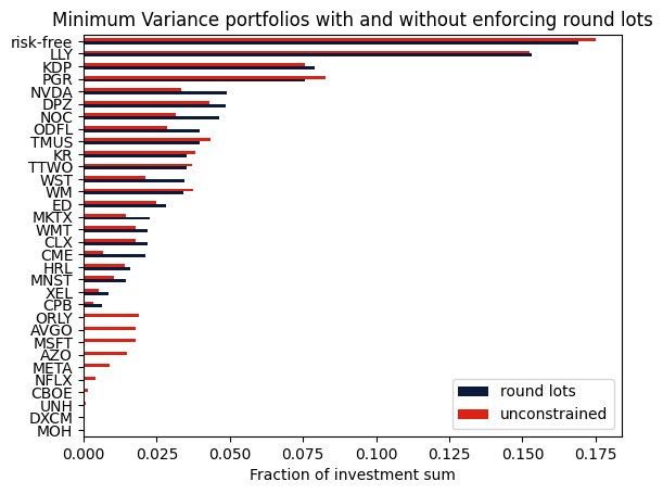
Comparison with the unconstrained portfolio
We can also compute and compare the portfolio without the minimum buy-in and lot constraints by changing the variable type and bounds of \(z\).
[13]:
x_lots = pd.concat([data["Position"], pd.Series([xrf.X], index=["risk-free"])])

# change type of z from semi-integer to continuous and lower bound to 0
df_model["z"].gppd.set_attr("vtype", gp.GRB.CONTINUOUS)
df_model["z"].gppd.set_attr("lb", 0)

m.params.OutputFlag = 0
m.optimize()

x_unconstr = pd.concat([df_model["x"].gppd.X, pd.Series([xrf.X], index=["risk-free"])])

# retrieve and display solution data
mask = (x_lots > 1e-5) | (x_unconstr > 1e-5)
df_data = pd.DataFrame(
    index=x_lots[mask].index,
    data={
        "round lots": x_lots[mask],
        "unconstrained": x_unconstr[mask],
    },
).sort_values(by=["round lots", "unconstrained"], ascending=True)

axs = df_data.plot.barh(color=["#0b1a3c", "#dd2113"])
axs.set_xlabel("Fraction of investment sum")
plt.title("Minimum Variance portfolios with and without enforcing round lots")
plt.show()
Takeaways
Data from pandas DataFrames can easily be used to build an optimization model via the
gurobipy-pandaspackage.To enforce buying round lots of shares, one needs to incorporate the asset price and the total investment amount into the model.
Minimum buy-in and round lot constraints can be modeled using semi-integer variables. Semi-integer variables are integer decision variables that may either take the value 0 or a value between specified bounds. They are a convenient tool to guarantee a minimum position size if an asset is bought.