Note
Download this Jupyter notebook and all
data
(unzip next to the ipynb file!).
You will need a Gurobi license to run this notebook, please follow the
license instructions.
Minimizing Variance
The standard mean-variance (Markowitz) portfolio selection model determines an optimal investment portfolio that balances risk and expected return. In this notebook, we minimize the variance (risk) of the portfolio, constraining the expected return to meet a prescribed minimum level. Please refer to the annotated list of references for more background information on portfolio optimization.
[2]:
import gurobipy as gp
import pandas as pd
import numpy as np
import matplotlib.pyplot as plt
Input Data
The following input data is used within the model:
\(S\): set of stocks
\(\mu\): vector of expected returns
\(\Sigma\): PSD variance-covariance matrix
\(\sigma_{ij}\) covariance between returns of assets \(i\) and \(j\)
\(\sigma_{ii}\) variance of return of asset \(i\)
[4]:
# Import example data
Sigma = pd.read_pickle("sigma.pkl")
mu = pd.read_pickle("mu.pkl")
Formulation
The model minimizes the variance of the portfolio, given that a prescribed minimum level of expected return is attained. Mathematically, this results in a convex quadratic optimization problem.
Decision Variables and Variable Bounds
The decision variables in the model are the proportions of capital invested among the considered stocks. The corresponding vector of positions is denoted by \(x\) with its component \(x_i\) denoting the proportion of capital invested in stock \(i\).
Each position must be between 0 and 1; this prevents leverage and short-selling:
Constraints
The budget constraint ensures that the entire capital is invested:
The expected return of the portfolio must be at least \(\bar\mu\):
Objective Function
The objective is to minimize the risk of the portfolio, which is measured by its variance:
Using gurobipy, this can be expressed as follows:
[5]:
mu_bar = 0.5  # Required return

# Create an empty optimization model
m = gp.Model()

# Add variables: x[i] denotes the proportion of capital invested in stock i
# 0 <= x[i] <= 1
x = m.addMVar(len(mu), lb=0, ub=1, name="x")

# Budget constraint: all investments sum up to 1
m.addConstr(x.sum() == 1, name="Budget_Constraint")

# Lower bound on expected return
ret_constr = m.addConstr(mu.to_numpy() @ x >= mu_bar, name="Min_Return")

# Define objective function: Minimize overall risk
m.setObjective(x @ Sigma.to_numpy() @ x, gp.GRB.MINIMIZE)
We now solve the optimization problem:
[6]:
m.optimize()
Gurobi Optimizer version 13.0.2 build v13.0.2rc1 (linux64 - "Ubuntu 24.04.4 LTS")

CPU model: AMD EPYC 7763 64-Core Processor, instruction set [SSE2|AVX|AVX2]
Thread count: 1 physical cores, 2 logical processors, using up to 2 threads

WLS license 2443533 - registered to Gurobi GmbH
Optimize a model with 2 rows, 462 columns and 924 nonzeros (Min)
Model fingerprint: 0x91dc4a17
Model has 0 linear objective coefficients
Model has 106953 quadratic objective terms
Coefficient statistics:
  Matrix range     [7e-02, 1e+00]
  Objective range  [0e+00, 0e+00]
  QObjective range [6e-03, 2e+02]
  Bounds range     [1e+00, 1e+00]
  RHS range        [5e-01, 1e+00]

Presolve time: 0.02s
Presolved: 2 rows, 462 columns, 924 nonzeros
Presolved model has 106953 quadratic objective terms
Ordering time: 0.01s

Barrier statistics:
 Free vars  : 461
 AA' NZ     : 1.070e+05
 Factor NZ  : 1.074e+05 (roughly 1 MB of memory)
 Factor Ops : 3.319e+07 (less than 1 second per iteration)
 Threads    : 1

                  Objective                Residual
Iter       Primal          Dual         Primal    Dual     Compl     Time
   0   8.01646707e+05 -8.01646707e+05  4.62e+05 2.79e-04  2.51e+05     0s
   1   2.62320026e+04 -2.76760257e+04  3.64e+03 2.20e-06  1.99e+03     0s
   2   4.08317831e+02 -2.00650283e+03  1.98e+01 1.19e-08  1.15e+01     0s
   3   1.67175634e+01 -1.37940884e+03  4.78e-01 2.89e-10  6.30e-01     0s
   4   2.23958857e+01 -4.30707773e+02  4.78e-07 3.33e-16  1.22e-01     0s
   5   1.92443494e+01  5.94640841e+00  5.77e-09 1.11e-16  3.59e-03     0s
   6   1.67030106e+01  1.38408810e+01  4.55e-10 2.22e-16  7.74e-04     0s
   7   1.52179879e+01  1.45858210e+01  4.67e-14 3.55e-15  1.71e-04     0s
   8   1.46942705e+01  1.46770325e+01  2.30e-13 2.87e-15  4.66e-06     0s
   9   1.46790601e+01  1.46790425e+01  6.18e-13 1.78e-15  4.75e-09     0s
  10   1.46790446e+01  1.46790446e+01  2.62e-13 6.86e-15  4.75e-12     0s

Barrier solved model in 10 iterations and 0.25 seconds (0.63 work units)
Optimal objective 1.46790446e+01
Display basic solution data:
[7]:
print(f"Minimum risk:     {m.ObjVal:.6f}")
print(f"Expected return:  {mu @ x.X:.6f}")
print(f"Solution time:    {m.Runtime:.2f} seconds\n")

# Print investments (with non-negligible value, i.e., > 1e-5)
positions = pd.Series(name="Position", data=x.X, index=mu.index)
print(f"Number of trades: {positions[positions > 1e-5].count()}\n")
print(positions[positions > 1e-5])
Minimum risk:     14.679045
Expected return:  0.500000
Solution time:    0.26 seconds

Number of trades: 8

TSLA    0.128472
AMD     0.017131
AVGO    0.070706
DXCM    0.035290
NFLX    0.051834
LLY     0.200962
ENPH    0.080654
NVDA    0.414950
Name: Position, dtype: float64
Efficient Frontier
The efficient frontier reveals the balance between risk and return in investment portfolios. It shows the best-expected risk level that can be achieved for a specified minimum return level. We compute this by solving the above optimization problem for a sample of admissible return levels.
[8]:
returns = np.linspace(0.21, 0.5, 20)
risks = np.zeros(returns.shape)
npos = np.zeros(returns.shape)

# Hide Gurobi log output
m.params.OutputFlag = 0

# Solve the model for each risk level
for i, ret in enumerate(returns):
    # Modify lower bound on expected return
    ret_constr.RHS = ret
    m.optimize()
    # Store data
    risks[i] = np.sqrt(x.X @ Sigma @ x.X)
    npos[i] = len(x.X[x.X > 1e-5])
We can display the efficient frontier to visualize the relationship between the expected return and the variance. We also display the relationship between the return and the number of positions in the optimal portfolio.
[9]:
fig, axs = plt.subplots(1, 2, figsize=(10, 3))

# Axis 0: The efficient frontier
axs[0].scatter(x=risks, y=returns, marker="o", label="sample points", color="Red")
axs[0].plot(risks, returns, label="efficient frontier", color="Red")
axs[0].set_xlabel("Standard deviation")
axs[0].set_ylabel("Expected return")
axs[0].legend()
axs[0].grid()

# Axis 1: The number of open positions
axs[1].scatter(x=returns, y=npos, color="Red")
axs[1].plot(returns, npos, color="Red")
axs[1].set_xlabel("Expected return")
axs[1].set_ylabel("Number of positions")
axs[1].grid()

plt.show()
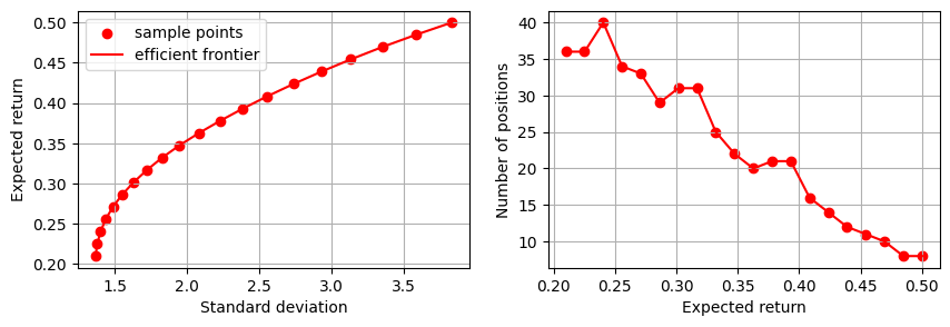
As expected, the number of open positions decreases as we enforce higher returns; the optimization will progressively invest in fewer high-risk but high-yield assets.